

Expert analysis at the intersection of AI, bioinformatics, and genomics. Breaking down the science shaping precision medicine — from whole-genome sequencing and liquid biopsy to spatial transcriptomics, proteomics, and metabolomics — grounded in peer-reviewed literature and written for the people building the next generation of life sciences products.
Search the blog by entering the keywords below and hitting “Enter“
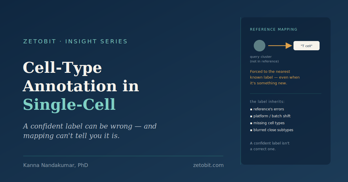
Cell-Type Annotation in Single-Cell RNA-Seq: Why a Confident Label Can Be Wrong, and Reference Mapping Can't Tell You It Is
Clustering gives you groups of cells; annotation gives them names — and that naming step feels like the objective payoff of the whole experiment. But every annotation method assigns a label by relating your cells to prior knowledge: a marker list, a reference atlas, a training set. It inherits that prior's limits without flagging them. The sharpest failure is structural: a standard classifier assigns every cell to one of the labels it was trained on, so a genuinely novel population gets forced to the nearest known type — confidently — instead of flagged as unknown. This piece covers the forced-label problem, why the reference isn't ground truth, and what defensible annotation requires.
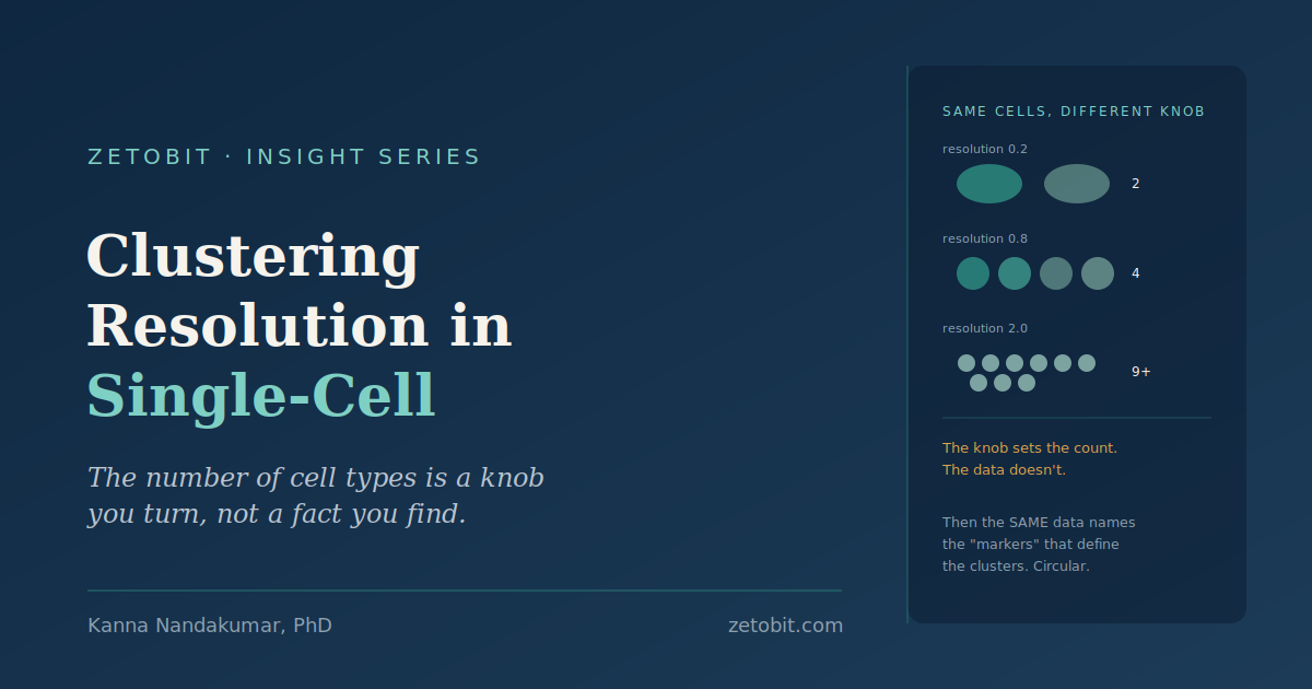
Clustering Resolution in Single-Cell RNA-Seq: Why the Number of Cell Types Is a Parameter You Choose, Not a Fact You Discover
Single-cell analysis answers "how many cell types are in this sample?" with an unsupervised clustering step — and it's the step most easily mistaken for objective. The number of clusters isn't something the data determines; it's set directly by a resolution parameter the analyst chooses. Turn it up and the same cells split into more groups, each with its own confident marker genes. Worse, those markers are tested on the same data used to draw the clusters — a circularity that inflates p-values even when there's only one true population. This piece covers over-clustering, the double-dipping problem, and how to tell a real cluster from a manufactured one.
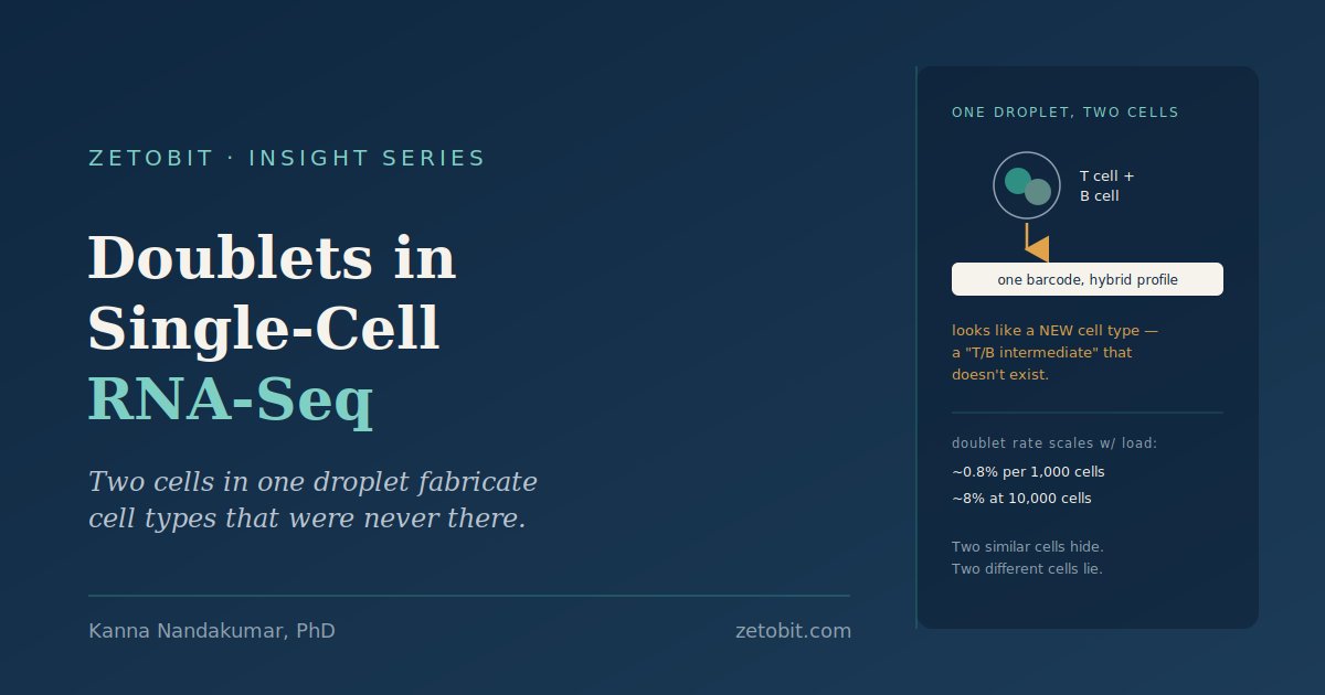
Doublets in Single-Cell RNA-Seq: Why Two Cells in One Droplet Fabricate Cell Types That Were Never There
The entire premise of single-cell RNA-seq is the word single: one droplet, one cell, one barcode. Doublets break it. When two cells share a droplet, their combined mRNA gets one barcode, and the analysis sees a single "cell" with a blended transcriptome. The danger is that the blend doesn't look like noise — it looks like a discovery. Two different cell types merged into one barcode land between their real clusters and read as a novel intermediate or transitional cell type that doesn't exist. This piece covers why the doublet rate is set when you load the chip, why detection is blind to same-type doublets, and what actually works.
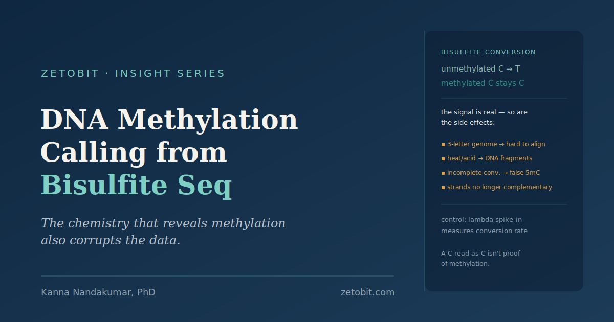
DNA Methylation Calling from Bisulfite Sequencing: Why the Chemistry That Reveals Methylation Also Corrupts the Data
Bisulfite conversion is an elegant trick: it rewrites unmethylated cytosines as thymines and leaves methylated ones untouched, turning an invisible epigenetic mark into a readable C-versus-T base change. But the same reaction fragments the DNA with heat and acid, collapses the four-letter genome to three letters (wrecking alignment), breaks strand complementarity, and — most dangerously — makes an unmethylated cytosine that escaped conversion indistinguishable from a truly methylated one. Incomplete conversion is a false-positive engine that only a spiked-in control can quantify. This piece covers why the chemistry that reveals methylation also corrupts the data, and what a trustworthy methylation pipeline requires.
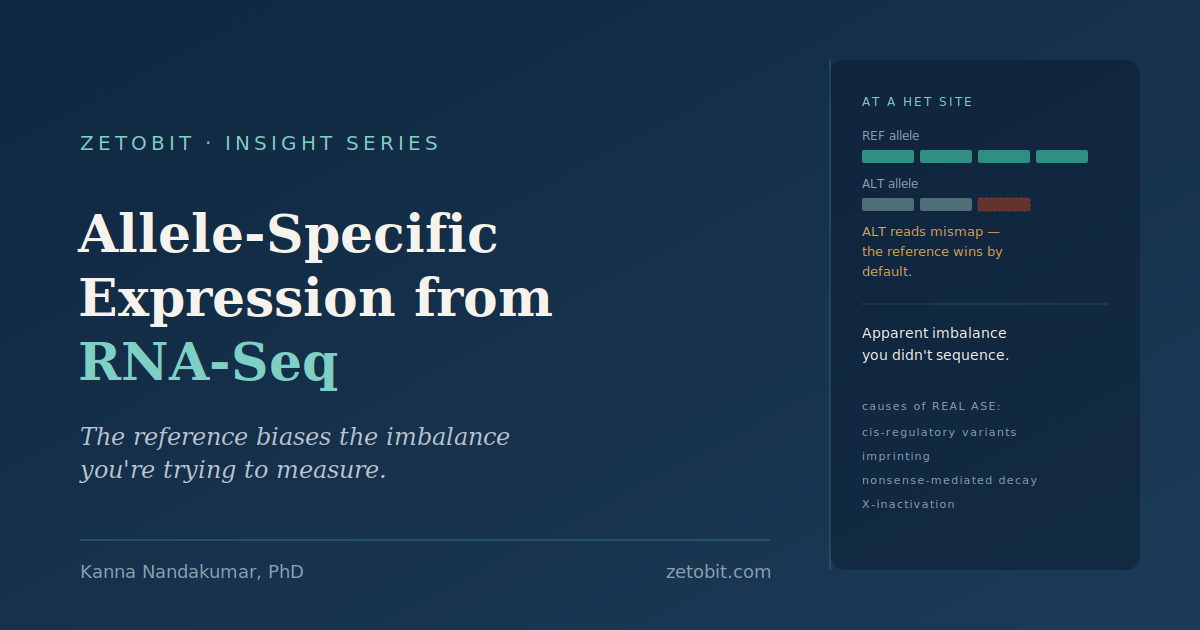
Allele-Specific Expression from RNA-Seq: Why the Reference Genome Biases the Very Imbalance You're Trying to Measure
Allele-specific expression asks a surgical question: within one sample, at a heterozygous site, is the maternal copy of a gene expressed as much as the paternal one? Because both alleles share a cell, any consistent imbalance points to a cis cause — a regulatory variant, imprinting, nonsense-mediated decay, X-inactivation — which makes ASE powerful where standard differential expression is blind. But the measurement has a thumb on the scale: reads are aligned to a reference that contains only one allele, so alternate-allele reads mismap more often and the reference count inflates. This piece covers reference bias, why correcting it is necessary but not sufficient, and what a trustworthy ASE pipeline requires.
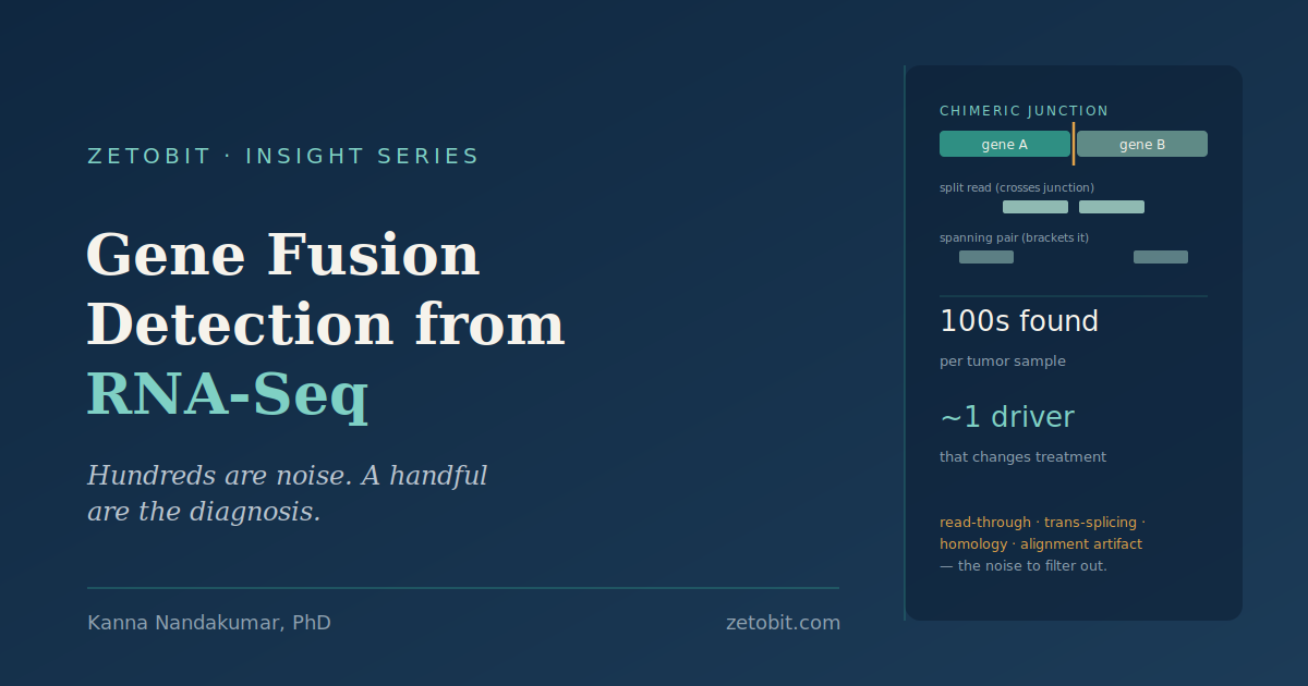
Gene Fusion Detection from RNA-Seq: Why Hundreds of Chimeric Transcripts Are Noise and a Handful Are the Diagnosis
An oncogenic gene fusion is one of the most actionable findings in cancer genomics — BCR::ABL1, ALK, RET, ROS1, NTRK each unlock a specific targeted therapy, and RNA-seq reads the fused transcript directly. But a single tumor sample yields hundreds of chimeric transcripts, and almost all are read-through transcription, normally-occurring chimeras, or alignment artifacts — not cancer. The clinical task isn't finding fusions; it's telling the one driver apart from the crowd of look-alikes, without discarding the real one in the process. This piece breaks down the read evidence, the structured false positives, why callers disagree, and what a real fusion pipeline has to do.
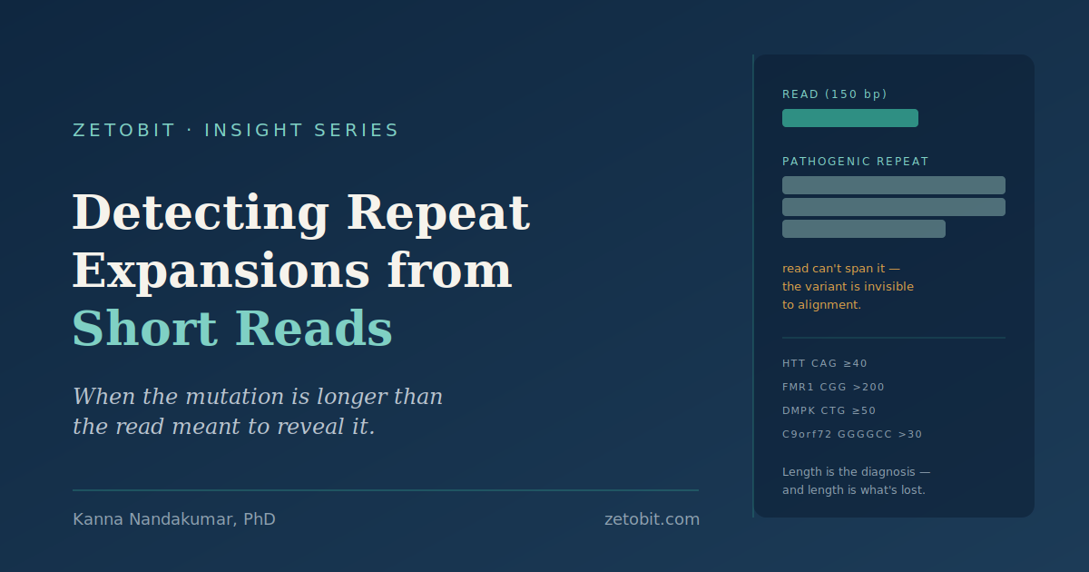
Detecting Repeat Expansions from Short Reads: Why the Pathogenic Allele Is Often Longer Than the Read That Should Reveal It
For a whole class of neurological diseases — Huntington's, fragile X, myotonic dystrophy, the ataxias, the commonest genetic ALS — the mutation isn't a changed base. It's a count: a short motif repeated too many times. And the pathogenic count is frequently longer than the 150 bp sequencing read that would need to contain it, so the very feature that makes the allele disease-causing is the feature that makes it invisible to a standard aligner. The pipeline reports the reference-length repeat, or nothing, and moves on — a false negative in exactly the disorders where the finding is decisive. This piece explains why, and what a real expansion-aware analysis requires.

Pharmacogenomic Star-Allele Calling: Why Clinical PGx Results Can't Be Read Off a VCF
A pharmacogenomic report answers a different question than a variant caller does. The clinician doesn't want a list of variants — they want a diplotype like CYP2D6 1/4, an activity score, a metabolizer phenotype, and a dose. A standard VCF can't deliver that. It lacks phase, so it can't say which variants sit together on the same chromosome to define an allele. It has no field for copy number, so gene duplications and deletions that flip a patient into ultrarapid territory go unrepresented. And a pseudogene next door corrupts the underlying SNVs. This piece explains why star-allele calling is a separate inference — and what a real PGx pipeline has to do.
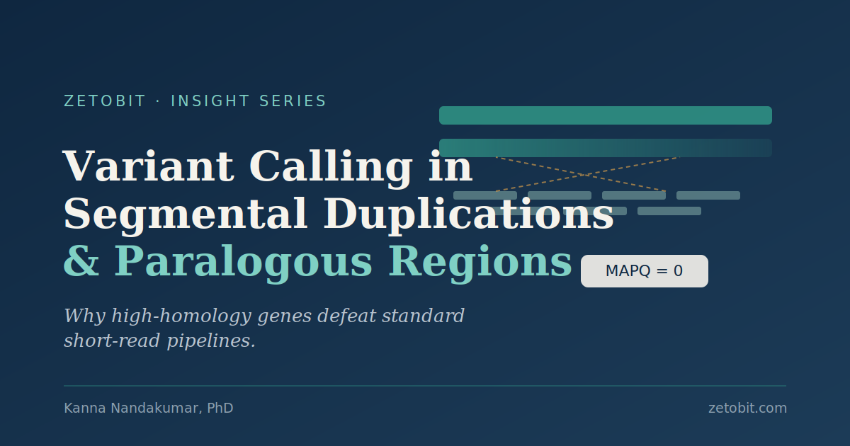
Variant Calling in Segmental Duplications and Paralogous Regions: Why High-Homology Genes Defeat Standard Short-Read Pipelines
A short-read pipeline reports clean genotypes across the exome, then goes silent at genes like PMS2, SMN1, and CYP2D6 — not for lack of a variant, but because it can't tell which locus the reads came from. Roughly 5–7% of the genome sits in segmental duplications overlapping 800+ genes, several clinically actionable. When reads map equally to a gene and its paralog, the aligner assigns MAPQ 0, and standard callers discard exactly those reads. The failure is invisible: coverage looks normal, no error is raised. This piece explains why the standard fixes backfire, what joint high-ploidy calling actually requires, and why declaring non-callability beats a silent dropout.
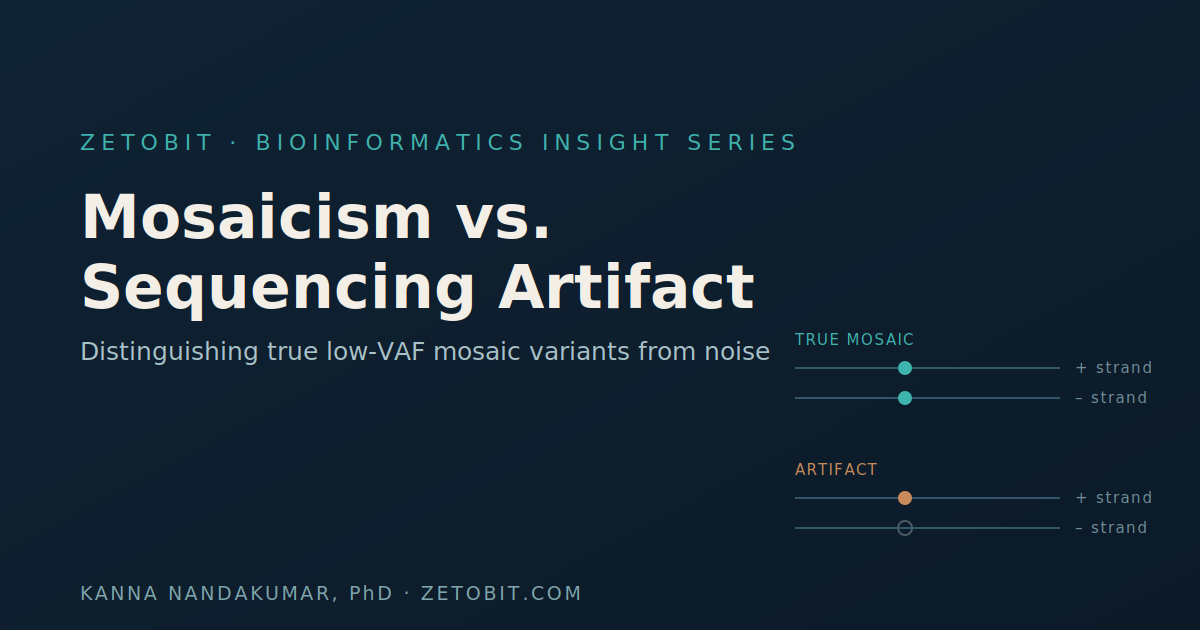
Mosaicism vs. Sequencing Artifact: Distinguishing True Low-VAF Variants from Noise
A germline heterozygous variant sits near 50% VAF — comfortably clear of the noise. Mosaic variants don't: a post-zygotic mutation present in a fraction of cells can sit at 2–5% VAF, right in the band where FFPE deamination, oxidative 8-oxoG damage, PCR errors, and mapping artifacts also live. A germline-tuned caller can't reliably tell them apart. This piece lays out the four signals that can — strand balance, substitution context, read-position and mapping quality, and molecular (UMI/duplex) consensus — surveys where mosaic callers like DeepMosaic and DRAGEN's mosaic mode stand, and gives a practical protocol for separating true low-VAF mosaicism from noise.
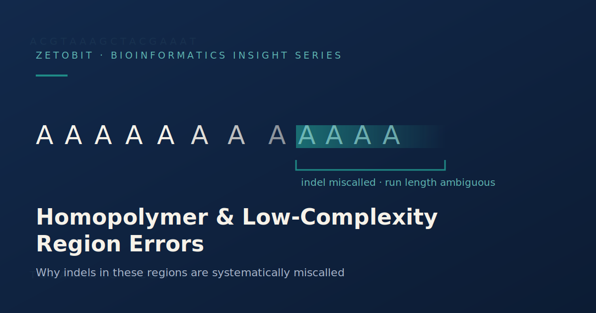
Homopolymer and Low-Complexity Region Errors: Why Indels in These Regions Are Systematically Miscalled
A run of eight identical bases isn't just harder to sequence than mixed sequence — it's harder in a way that biases the answer. Indel errors in homopolymers and low-complexity regions aren't random noise: they concentrate in predictable places, they favor certain lengths, and they survive filtering. This piece traces the failure through the whole pipeline — polymerase slippage that miscounts the run, aligners with no unique place to anchor a gap, and callers whose confidence inflates rather than degrades on biased evidence. Crucially, more coverage doesn't rescue you. What does: canonical normalization, context-aware error models, stratified validation, and flagging long-run indels for orthogonal confirmation.
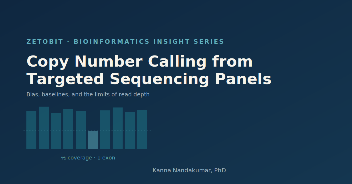
Copy Number Calling from Targeted Sequencing Panels: Bias, Baselines, and the Limits of Read Depth
A single-exon deletion lands in a clinical report with clean-looking evidence: coverage drops to half over the exon, exactly what a heterozygous loss should produce. Six weeks later, orthogonal MLPA comes back normal. Nothing was deleted — the panel measured a dip in capture efficiency and called it biology. Targeted panels are an impoverished substrate for copy number: no genome-wide baseline, GC and probe-level biases that mimic deletions, and single-exon calls that compete directly with noise. This piece walks through why depth isn't copy number, the three biases that masquerade as losses, and what actually earns a confident CNV call.
The Sample You Think You Sequenced
Every variant call rests on an unstated premise: the reads in this BAM came from one person — the right person. Contamination and sample swaps break that premise silently. There's no error message for a tube mix-up and no alignment flag when 2% of reads belong to someone else; the pipeline runs cleanly and hands you variants that look like real biology. This piece walks through the three failure modes — cross-sample contamination (VerifyBamID2's FREEMIX), tumor–normal swaps and low-level contamination (Conpair, reliable to 0.1%), and cross-species contamination in xenografts — and why each belongs as a QC gate before interpretation, not a post-hoc audit.
The Reads That Missed on Purpose
Every hybrid-capture assay has a shadow: the reads that landed outside the target. In a typical panel or exome run that shadow is a large fraction of the data — usually discarded as wasted sequencing. But off-target reads are ultra-low-depth whole-genome sequencing you've already paid for. Read as a trend, the off-target fraction flags capture and protocol drift and tightens contamination estimates that gate low-VAF reporting. Read as signal, it rescues copy-number calls beyond the target, HRD and tumor-fraction scores, and off-panel loci like mitochondrial pharmacogenetic variants. The catch: it carries genome-scale signal, not base-level calls. Match the question to the resolution.
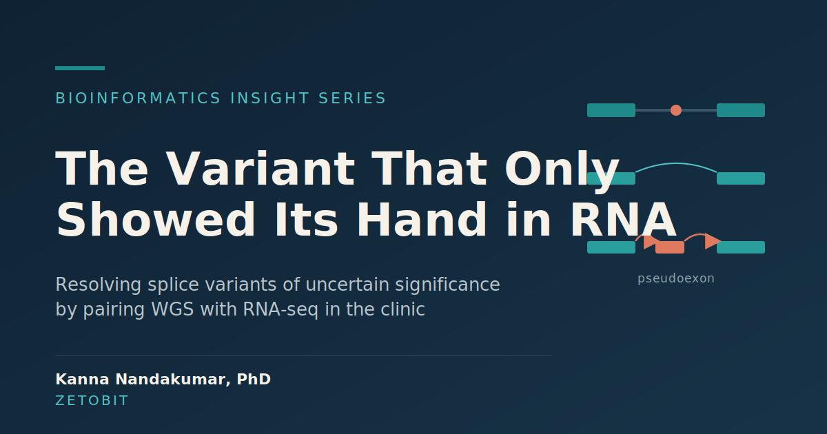
The Variant That Only Showed Its Hand in RNA
A whole-genome report comes back clean on the known genes, and the case stalls on a variant sitting 150 bases deep in an intron — silent by every coding metric, flagged by a prediction tool with a score that could mean anything. On DNA alone, it's unresolvable. This installment is a detailed look at the one clinical niche where pairing WGS with RNA-seq truly earns its cost: resolving the deep-intronic and synonymous splice variants that WGS is uniquely good at finding and uniquely bad at interpreting. How the two assays work in a loop, the three RNA-seq signals that carry the evidence, and where the pairing quietly fails.
The Allele That Never Aligned
Every RNA-seq experiment measures expression against a reference that is, by construction, somebody else's genome — and the aligner is not neutral about it. A read carrying a non-reference allele arrives already penalized, already slightly less likely to survive. Multiply that across every heterozygous site and you get a systematic distortion with a known sign: reference alleles look more expressed than they are. Degner's 2009 work found that filtering biased sites eliminated 40% of top ASE signals. At HLA, 18.6% of 1000 Genomes genotype calls were simply wrong. Insight Series No. 17 covers where the bias concentrates, what actually fixes it, and why sequencing deeper does not.
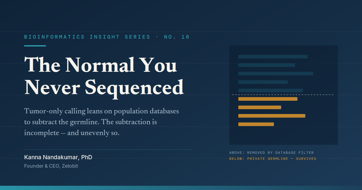
The Normal You Never Sequenced
Tumor-only sequencing is the reality for archival blocks, constrained consent, and single-library budgets — and when the matched normal is missing, a population database gets drafted in as the control. It isn't one. Private germline variants, the ones gnomAD has never seen, survive filtering wearing exactly the same clothes as real somatic mutations. The published positive predictive value of database filtering runs 35–62% for European-ancestry samples and 20–40% for Hispanic, African American, and African ancestry samples: a call set where errors can outnumber truth, skewed against the patients genomics already serves worst. Insight Series No. 16 covers what the filter misses, why ancestry drives it, and what to build instead.
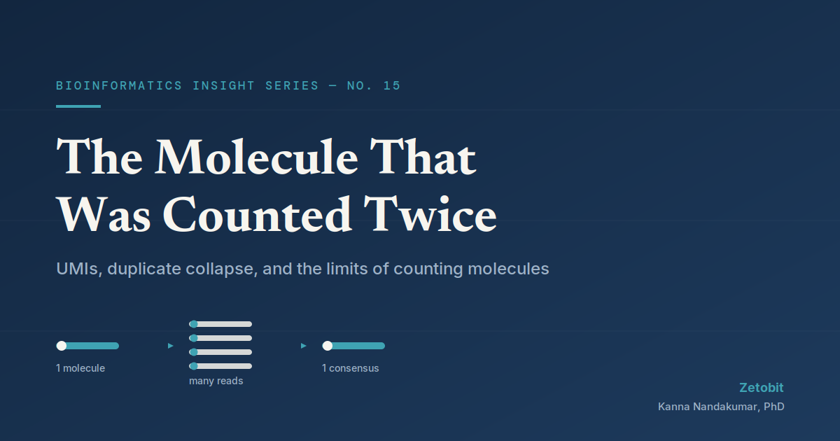
The Molecule That Was Counted Twice
A variant appears at 0.4% allele frequency - fourteen alternate reads out of thirty-five hundred. Whether that reaches a report depends on a question read counts cannot answer — how many molecules do fourteen reads represent? Unique molecular identifiers exist to answer it, and when they work, they work extraordinarily well. But the tag-collapse-count logic hides assumptions that fail quietly: barcodes collide, barcodes mutate, and every consensus threshold you raise discards the molecules that were your sensitivity. Beneath it all sits a limit no amount of sequencing can move — you cannot detect a molecule that was never in the tube.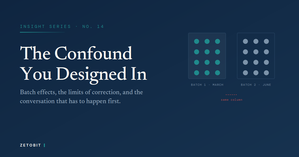
The Confound You Designed In
Every sequencing experiment has batches. Samples run on different days, on different flow cells, with different reagent lots. That's unavoidable. What's avoidable is confounding those batches with the thing you're trying to measure — and that mistake gets made at the bench, weeks before anyone opens R.
The question that reaches me is usually "which correction method should we use?" Often it has no good answer. ComBat will produce output. So will every other method. None will produce truth, because the information needed to separate technical from biological signal was never collected.
Correction is not a repair mechanism. Here's what is.
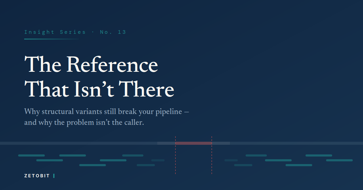
The Reference That Isn't There
Short reads gave us a decade of clean SNV calling and an illusion of completeness. The illusion holds until you ask what happened to a 4 kb region — then the pipeline that called your missense variant with 99% confidence goes quiet.
Structural variants account for more variable base pairs per genome than SNVs and indels combined, yet they sit exactly where our tooling is weakest: repeat-flanked regions where short reads cannot map uniquely. Swapping callers won't fix it. The deeper problem is a linear reference that structurally cannot represent the thing being measured.
Here's what that means for a production pipeline.