

Expert analysis at the intersection of AI, bioinformatics, and genomics. Breaking down the science shaping precision medicine — from whole-genome sequencing and liquid biopsy to spatial transcriptomics, proteomics, and metabolomics — grounded in peer-reviewed literature and written for the people building the next generation of life sciences products.
Search the blog by entering the keywords below and hitting “Enter“
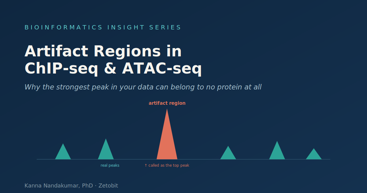
Artifact Regions in ChIP-seq and ATAC-seq: Why the Strongest Peak in Your Data Can Belong to No Protein at All
A handful of regions in every genome accumulate enormous sequencing signal in every experiment — whatever antibody, whatever cell type, whatever you were looking for. A peak caller can't tell that signal from a real binding event, so it reports these artifacts as your most confident peaks. They come from low-mappability, repeat-rich, and assembly-gap regions, run up to ~6400× background, and can hold over 20% of all reads. Worse, they're reproducible across samples and studies — the usual evidence for a real signal. This piece explains the ENCODE blacklist, why input controls and blacklist masking are both non-optional, and why an artifact map is specific to an assay and an assembly.
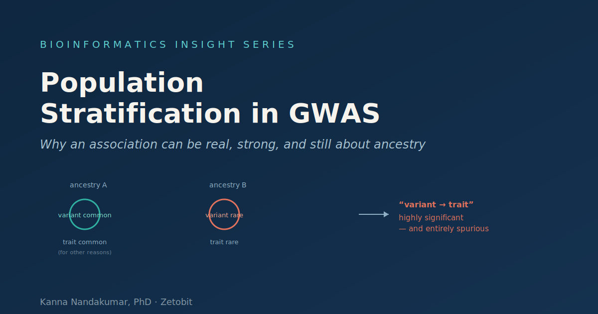
Population Stratification in GWAS: Why an Association Can Be Real, Strong, and Still About Ancestry
A GWAS can hand you a variant with a crushing p-value that replicates in a second cohort and still has nothing to do with the trait. If ancestry differs between cases and controls, the association test faithfully reports ancestry as biology — a variant only needs to differ in frequency across ancestral groups while the trait also differs across them, often for non-genetic reasons. The variant need not be functional or near any causal locus (the "chopstick gene" problem). This piece explains how stratification manufactures strong, reproducible false positives, how QQ plots, λ, PCA, and LD score regression detect and correct it — and why the corrections have their own failure modes.
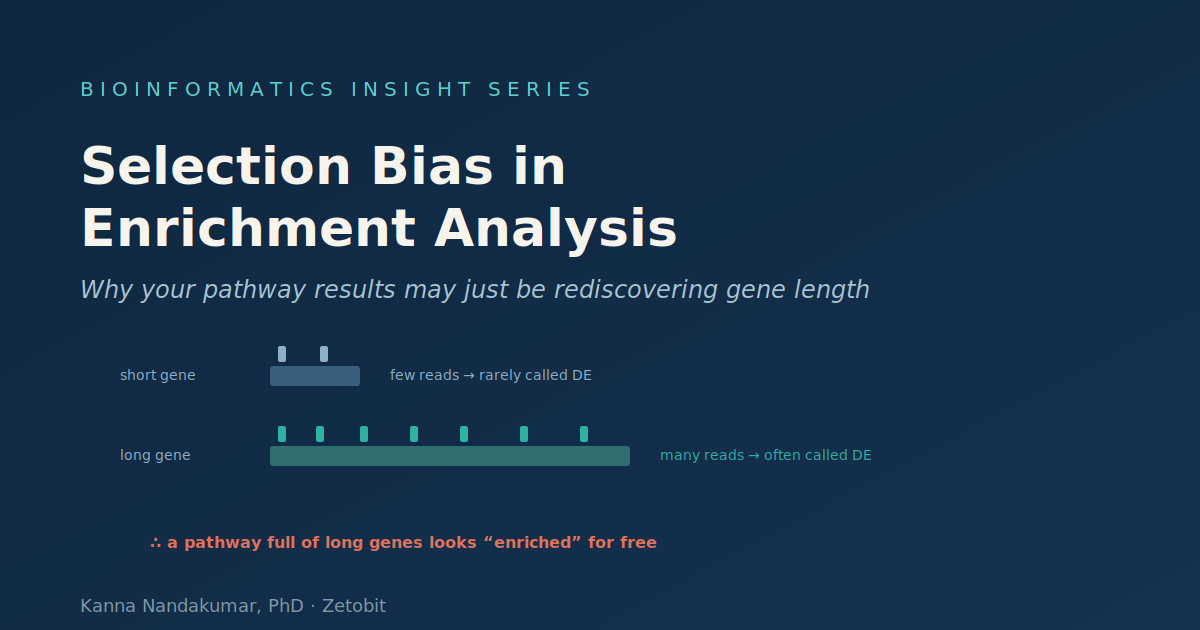
Selection Bias in Enrichment Analysis: Why Your Pathway Results May Just Be Rediscovering Gene Length
GO and pathway enrichment turns a list of differentially expressed genes into a biological story — and it feels like the safe, mechanical part of the analysis. It isn't. The standard test assumes every gene is equally likely to be called differentially expressed, and RNA-seq breaks that: longer, more highly expressed genes accumulate more reads and more statistical power, so they're called DE more often. Any pathway full of long genes then lights up as "enriched" for free — and long genes cluster in exactly the interesting-sounding categories. This piece explains the length-bias trap, the background-set trap, and how to correct both.
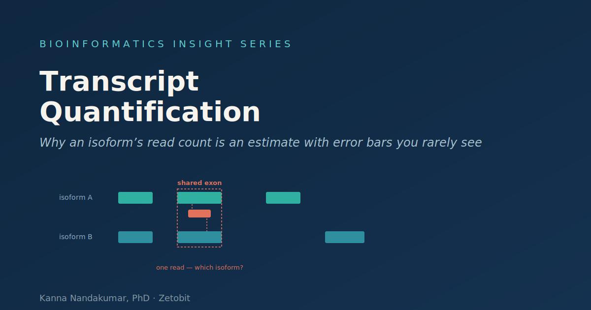
Transcript Quantification: Why an Isoform’s Read Count Is an Estimate With Error Bars You Rarely See
A gene's isoforms are built from overlapping exons, so most reads can't be pinned to a single transcript — they're compatible with several. Salmon and kallisto resolve that by splitting shared reads probabilistically and reporting one clean TPM per isoform. But that number is a point estimate of a quantity the reads may not have determined: an isoform with its own unique reads is trustworthy, while one whose reads are all shared with siblings gets the same tidy value with enormous hidden uncertainty. This piece explains why transcript-level counts are softer than gene-level, why they break gene-level DE tools, and how inferential replicates recover the missing error bars.
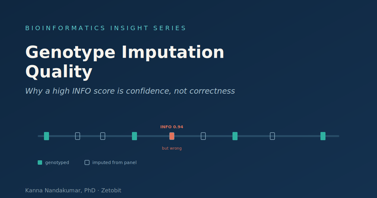
Genotype Imputation Quality: Why a High INFO Score Is Confidence, Not Correctness
Imputation turns a few hundred thousand genotyped SNPs into tens of millions, filling the gaps from a reference panel and stamping each variant with an INFO or Rsq quality score. The trap is what that score measures: the model's certainty about its own guess, computed without ever seeing a true genotype — not whether the guess is right. Confidence and accuracy agree for common variants but diverge exactly where imputation is hard: rare variants (true accuracy falls off a cliff the score doesn't show) and ancestry-mismatched panels. This piece explains why a high INFO score is confidence, not correctness — and what to check instead.
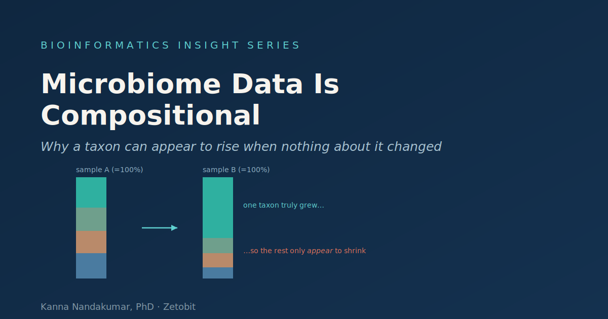
Microbiome Data Is Compositional: Why a Taxon Can Appear to Rise When Nothing About It Changed
Microbiome sequencing doesn't count bacteria — it reports each taxon's share of a fixed pool of reads, and those shares are forced to sum to one. That single constraint quietly manufactures false findings: correlations biased negative even for independent taxa, and long lists of taxa that "significantly decrease" when the only real event was one organism blooming and squeezing everyone else's slice. Rarefying and subsetting don't fix it. This piece explains the constant-sum constraint, why log-ratio methods like ALDEx2 and ANCOM are the honest alternative, and why answering an absolute question needs an external anchor like qPCR or a spike-in.
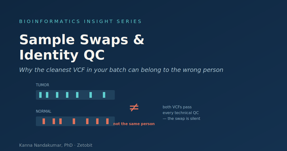
Sample Swaps and Identity QC: Why the Cleanest VCF in Your Batch Can Belong to the Wrong Person
A mislabeled tube, a pipetting error, a transposed row on a plate — and a sample produces a flawless VCF that belongs to someone else, or to two people at once. Every technical metric passes, because technically nothing failed: read quality, coverage, Ts/Tv are all normal. Standard QC is structurally blind to it, because those metrics ask "did the sequencing work?" not "is this the right person?" The only check that catches a swap is a genetic fingerprint — genotyping a panel of common SNPs to ask the genome who it belongs to. This piece explains why identity is a separate QC axis, and why tumor-normal work is especially exposed.
RNA Velocity: Why a Confident Arrow of Cellular Direction Can Point the Wrong Way
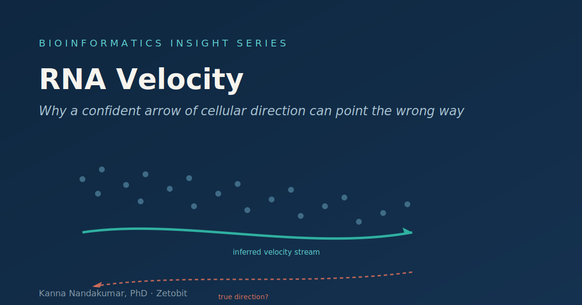
RNA velocity promises what a static snapshot can't give: the direction each cell is heading, inferred from the ratio of unspliced to spliced RNA. The arrows are visually compelling and often biologically right — but they rest on kinetic assumptions real data frequently violates (genes with multiple rate kinetics can produce distorted or even reversed velocity), the unspliced signal is faint and noisy, and the smooth streamline you see can be manufactured by the 2D projection rather than read from the biology. One critique produced a coherent-looking flow from three genes with no directional signal at all. This piece explains why a clean velocity stream is a hypothesis, not a measurement.
Variant Normalization: Why the Same Variant Written Two Ways Silently Fails to Match
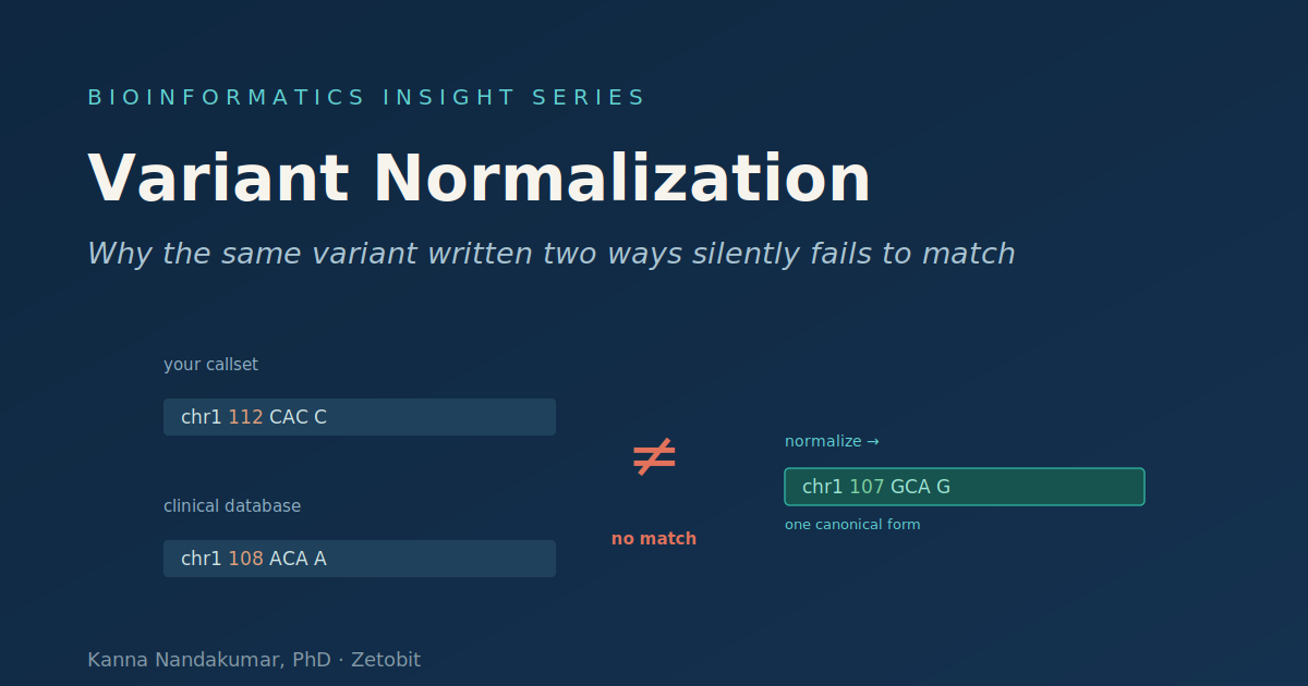
A single insertion or deletion can be written in several equally correct VCF representations — different position, different alleles, same biological edit. To a human they're obviously identical. To a computer doing an exact match against ClinVar, they're different variants, and the mismatch is completely silent: every job runs, every file is well-formed, and a pathogenic variant simply fails to annotate. This piece explains why VCF doesn't enforce a unique spelling, how left-alignment and parsimony produce one canonical form (and the uniqueness theorem that makes matching correct), why multiallelic decomposition is a required partner step, and why two different normalizers can still disagree on indels in repeats.
False Positives in Metagenomic Classification: Why a Handful of Reads Can Invent a Pathogen That Was Never There
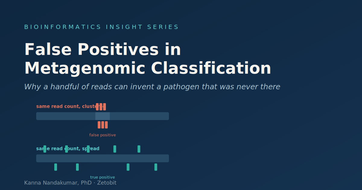
In metagenomic pathogen detection the organism you're hunting may be fewer than 100 reads out of tens of millions — and contamination, a conserved rRNA gene, or a dirty database entry can produce exactly that same handful. Read count alone cannot tell the real signal from the manufactured one. This piece explains why the instinctive metric fails at low abundance, why false-positive reads share a geometry (they pile up in the same few spots while real organisms spread across the genome), and how unique-k-mer counting operationalizes breadth of coverage — the KrakenUniq threshold of ~1000 unique k-mers eliminated many background pathogen identifications that a read-count filter would have passed.
HLA Typing from Short Reads: Why the Most Polymorphic Region in the Genome Defeats Standard Alignment
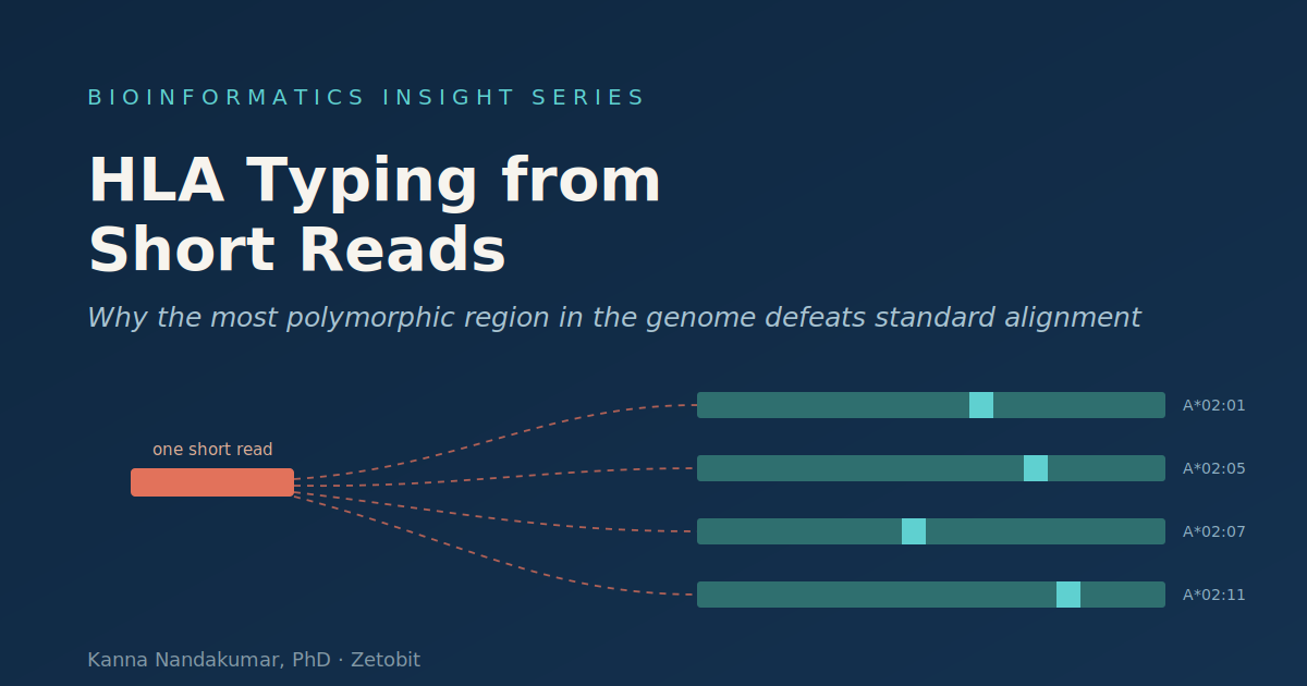
Typing HLA is not variant calling. It's choosing two alleles out of thousands whose sequences differ by less than the ambiguity of a single short read — against a reference database that is itself incomplete. That's why a pipeline that nails the rest of the genome can quietly return the wrong HLA type. This piece walks through why the standard align-to-GRCh38-and-call workflow fails at the MHC, why four-digit resolution collapses on short reads (one early method got only ~32% of four-digit class I calls right), why low-SNP-density loci like DQA1/DPA1/DPB1 can't be phased, and how the working tools model the ambiguity instead of ignoring it.
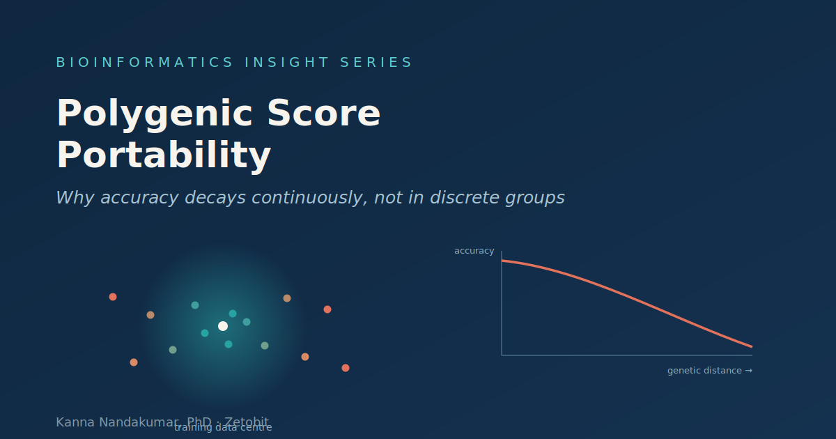
Polygenic Score Portability Across Ancestries: Why Accuracy Decays Continuously and a Population Label Cannot Tell You Where
A polygenic score trained in one population predicts poorly in another — that much is well known. What's less appreciated is that the loss isn't a step change between labeled groups. It's a smooth decline with genetic distance from the training data, and it happens inside a single ancestry label as surely as across the boundary between two. A large biobank analysis found accuracy correlates −0.95 with genetic distance across 84 traits, and the closest Hispanic/Latino individuals can be predicted as well as the farthest Europeans. This piece explains why the population label is the wrong unit — and what to report instead.
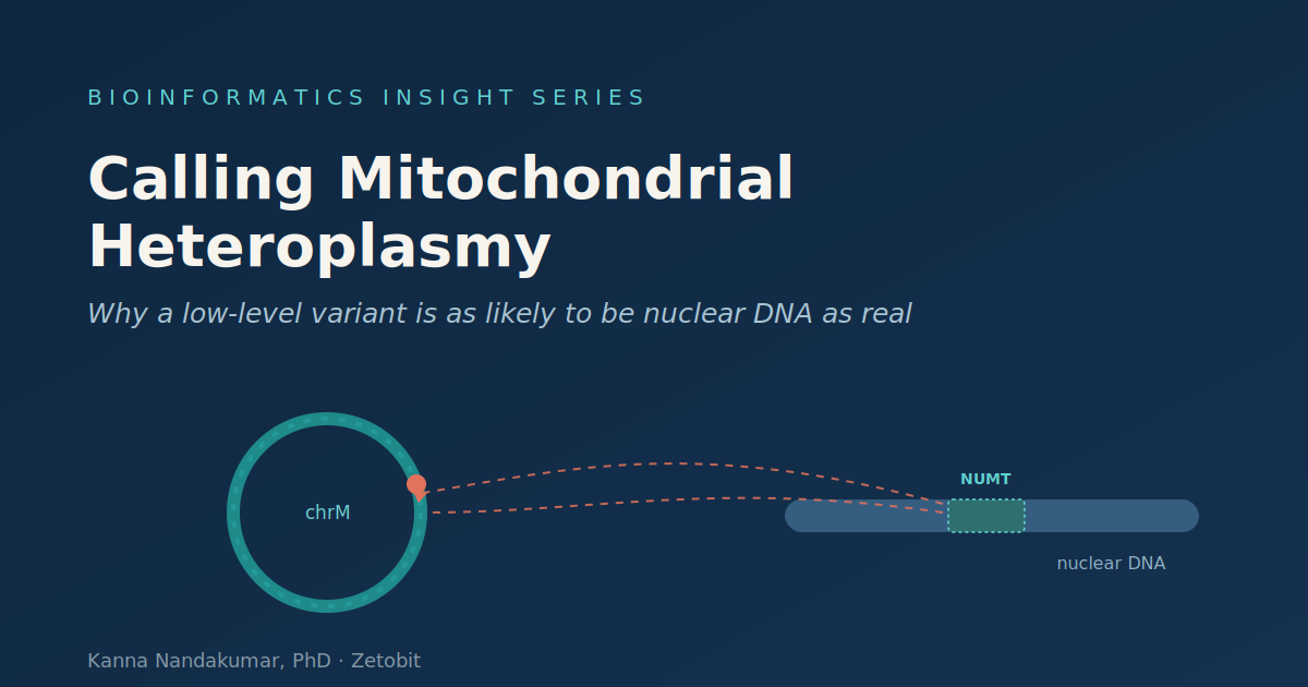
Calling Mitochondrial Heteroplasmy: Why a Low-Level Variant Is as Likely to Be Nuclear DNA as Real
Point a germline pipeline at chrM and it runs without complaint and hands you a VCF. That's the problem. The mitochondrial genome breaks nearly every assumption a standard variant caller is built on — it's circular, it carries a variant at any fraction rather than two clean alleles, and, most treacherously, fragments of it are scattered across the nuclear genome as NUMTs. Reads from those nuclear copies mis-map onto the mitochondrial reference and manufacture low-heteroplasmy variants that were never in a mitochondrion. Worse, whether they clear your threshold depends on the sample's mtDNA copy number. This piece covers why a flat cutoff is the wrong instinct, and what actually controls the confound.
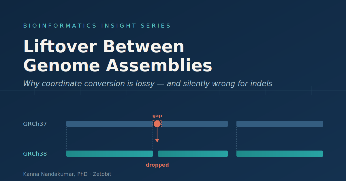
Liftover Between Genome Assemblies: Why Coordinate Conversion Is Lossy and Silently Wrong for Indels
Moving a variant from GRCh37 to GRCh38 looks like arithmetic on a position — pass the coordinates through a chain file and you're done. It isn't that simple. A genome assembly is a specific reconstructed sequence, not a neutral ruler, and wherever two builds spell the same variant with different alleles, the standard liftover tools quietly drop it or convert it into a record that will never match a natively called genome. SNVs mostly survive; indels and short-tandem-repeat variants are where it breaks, silently. This piece walks through what a chain file actually encodes, why tool choice isn't cosmetic, and when you should realign instead of lift over.

Panel vs. Exome vs. Genome: Why More Sequencing Isn't Always More Answers
It's tempting to treat panel, exome, and genome as a ladder — more territory, more diagnoses, strictly better if you can afford it. But breadth trades against depth, interpretability, turnaround, and the burden of uncertain and incidental findings — and the widest test isn't always the one that answers your question. A deep panel can out-diagnose an exome for a well-defined phenotype; a uniform genome can out-detect a patchy exome for the right coding variant. This piece frames test selection as a design decision driven by the question — the phenotype's specificity, the likely variant class, and the reporting strategy — not a reflex toward "more."
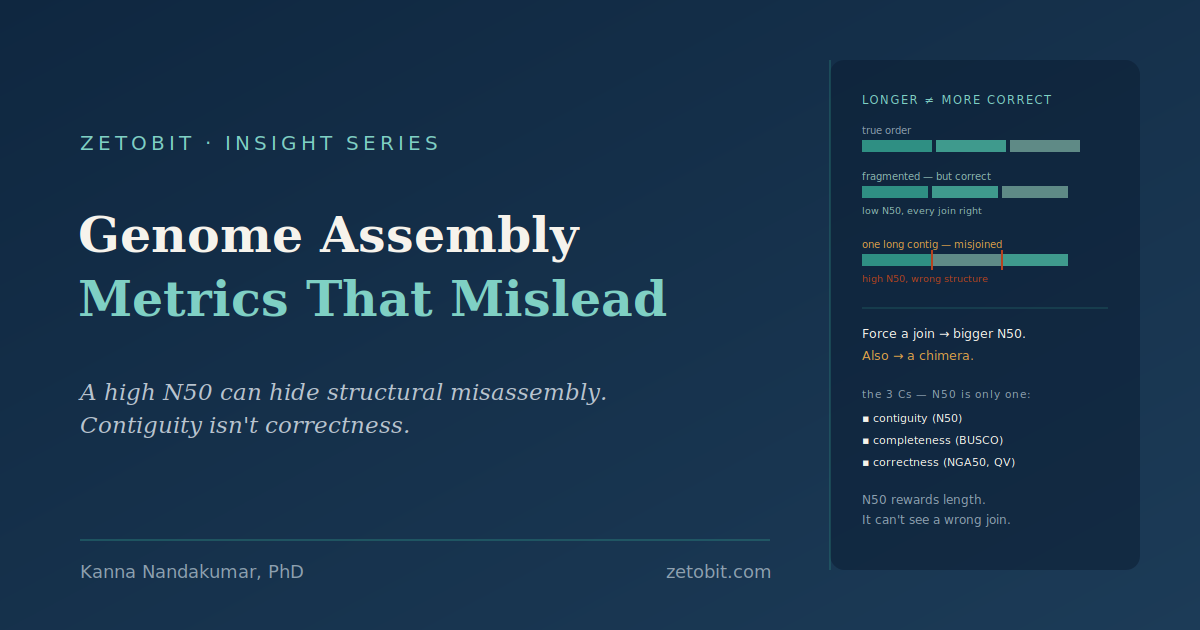
Genome Assembly Metrics That Mislead: Why a High N50 Can Coexist With Structural Misassemblies
N50 is the number everyone quotes to prove a genome assembly is good: the bigger it is, the more contiguous the assembly. But N50 measures only how long the pieces are — not whether they're joined correctly. And the fastest way to raise it is to make exactly the kind of aggressive join that produces a chimera. A misjoin fuses two sequences that don't belong adjacent into one longer contig, which raises N50 — the structural error and the metric improvement are the same event. This piece covers the three Cs of assembly quality, why contiguity isn't correctness, and how to actually verify structure.
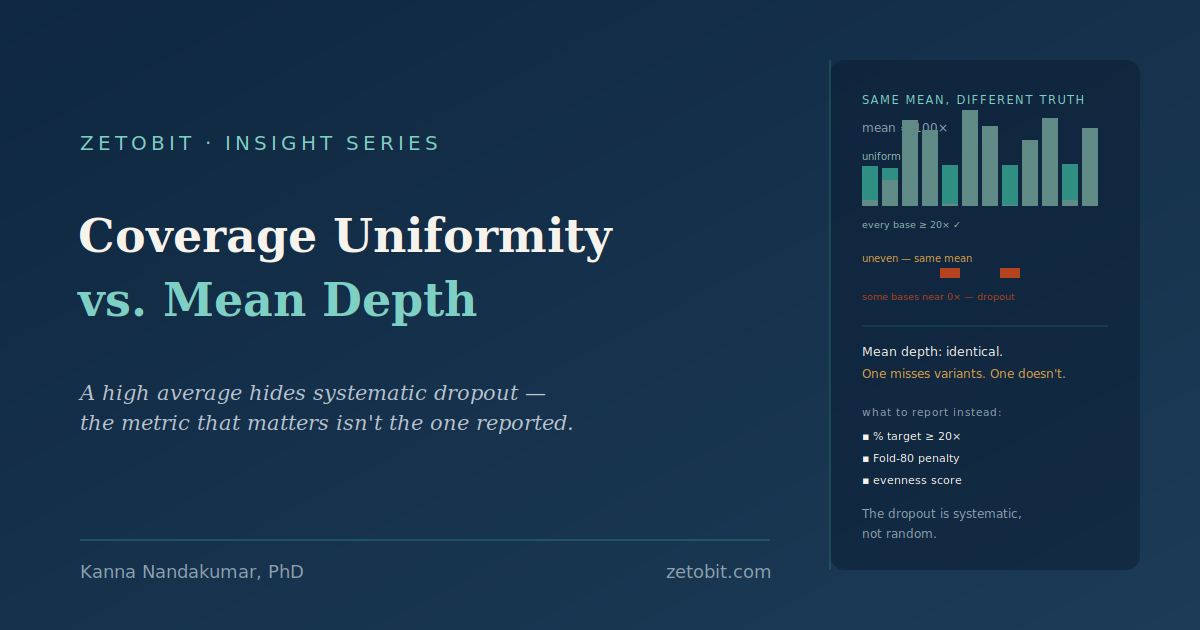
Coverage Uniformity vs. Mean Depth: Why the Average That Reassures You Hides the Dropout That Fails the Sample
"Sequenced to 100× mean coverage" sounds like every base was read a hundred times. It wasn't. Mean depth is an average over a distribution, and two samples with the same average can differ enormously in whether a given clinically important base was covered at all — because sequencing dropout is systematic, not random. GC-extreme regions, promoters and first exons, long exons, and repeats drop out in the same places every run, invisible in the mean. This piece covers why the average reassures while the distribution decides which variants get called, and which uniformity metrics — percent-above-threshold, Fold-80, evenness — actually capture what the mean hides.

Phasing and Haplotype Assembly Limits: Why "Phased" Has a Resolution You Rarely See Reported
A phased genome sounds like a solved genome — two clean parental haplotypes, allele by allele. In reality "phased" means the chromosome was broken into blocks: contiguous stretches the method declares internally phased, separated by gaps it couldn't resolve, each carrying its own error rate, with no reliable phase relationship between blocks. The single number usually reported — block N50 — describes only how long the blocks are, not whether they're correct. And a switch error, one wrong junction, inverts every allele downstream of it, silently flipping a compound-heterozygote call from benign to disease-causing. This piece covers switch vs. flip errors, block boundaries, and the resolution "phased" hides.
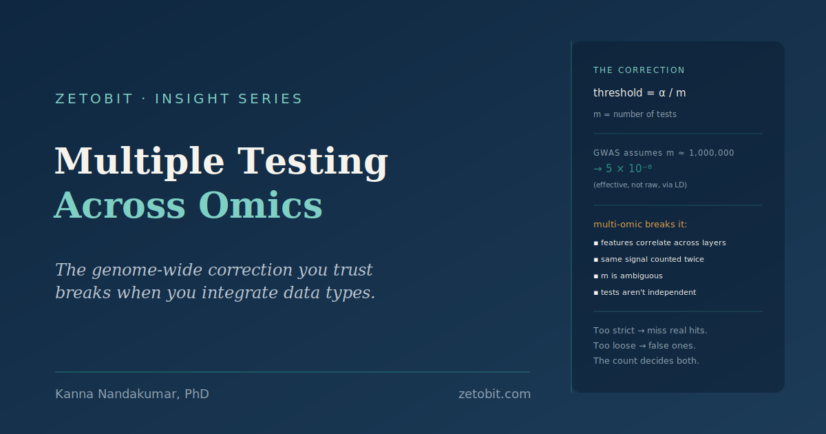
Multiple Testing Across Omics: Why the Genome-Wide Correction You Trust Breaks When You Integrate Data Types
The GWAS threshold of 5×10⁻⁸ feels like a constant of nature. It isn't. It's a Bonferroni correction — 0.05 divided by roughly a million effectively independent tests, a count derived from the genome's linkage-disequilibrium structure. That works because the dependence is understood and confined to one data type. Multi-omic integration removes both comforts: you're testing SNPs, transcripts, proteins, and metabolites with different feature counts, different correlation structures, and correlations between them. The number of tests — the denominator every correction depends on — stops having a clean answer, and the same biological signal gets counted once, thrice, or not at all. This piece covers why.
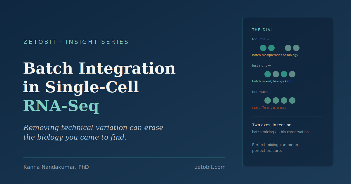
Batch Integration in Single-Cell RNA-Seq: Why Removing Technical Variation Can Erase the Biology You Came to Find
Combining single-cell datasets from different runs, labs, or chemistries means removing the technical batch effects between them. But technical and biological variation are entangled in the same numbers, and no algorithm separates them perfectly. Integration is a balancing act between two goals that pull in opposite directions — mixing the batches together vs. conserving real biology — with a dangerous failure mode: push too hard toward blending, and you don't just remove noise, you erase genuine differences. And because the output is a clean, well-mixed embedding, the erasure is invisible. This piece covers the tradeoff, why over-correction is common, and the confounding trap where batch IS the biology.