


Expert analysis at the intersection of AI, bioinformatics, and genomics. Breaking down the science shaping precision medicine — from whole-genome sequencing and liquid biopsy to spatial transcriptomics, proteomics, and metabolomics — grounded in peer-reviewed literature and written for the people building the next generation of life sciences products.
Search the blog by entering the keywords below and hitting “Enter“
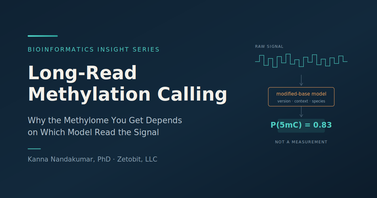
Long-Read Methylation Calling: Why the Methylome You Get Depends on Which Model Read the Signal
Bisulfite sequencing converts unmethylated cytosine chemically, so the methylation state is written into the sequence and read out like any other base. Long-read platforms don't convert anything — they record the raw current and hand it to a neural network that returns a probability the base was modified. That's a different kind of claim. Swapping the model changes the methylome without changing the DNA: an independent July 2026 evaluation found the newest high-accuracy model did not always beat its predecessor, and a purpose-built plant model improved CHH correlations by up to 118% over the general-purpose one.
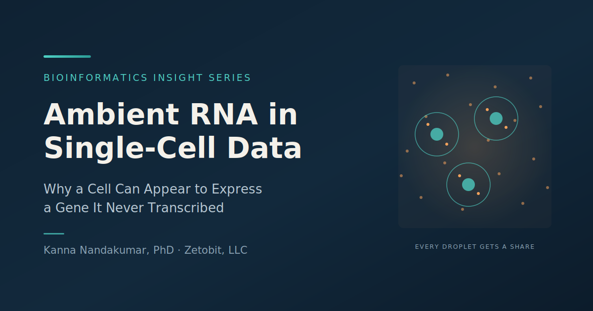
Ambient RNA in Single-Cell Data: Why a Cell Can Appear to Express a Gene It Never Transcribed
Dissociation ruptures cells, and their mRNA goes into the suspension. Every droplet that captures a cell also captures a sample of that free-floating pool, and those molecules are counted against the cell's barcode. It isn't random noise — it's a systematic addition weighted toward whatever the most abundant cells were transcribing, applied to every cell in the experiment. Contamination ranges from 2% to 50% across experiments. In brain single-nucleus data, all glia carry neuronal ambient RNA, and roughly 80% of the markers defining a published "immature oligodendrocyte" population turned out to be ambient transcripts. The cell type dissolved on reanalysis.

Clonal Hematopoiesis as a Confounder: Why a Variant Can Be Somatic and Still From the Wrong Tissue
Every QC mechanism a somatic pipeline has is designed to answer one question: is this variant real? Clonal hematopoiesis defeats all of them by satisfying the criterion. A CH variant is a genuine somatic mutation, present in the specimen, reproducible on orthogonal testing, correctly called — and not from the tumor. In one deep-sequencing study, 81.6% of cfDNA mutations in controls and 53.2% in cancer patients had features consistent with clonal hematopoiesis. Across 16,812 liquid profiles, 39% of detected BRCA2 variants were of CH origin. The pipeline has no filter for provenance, because provenance was never something a variant caller was asked to determine.
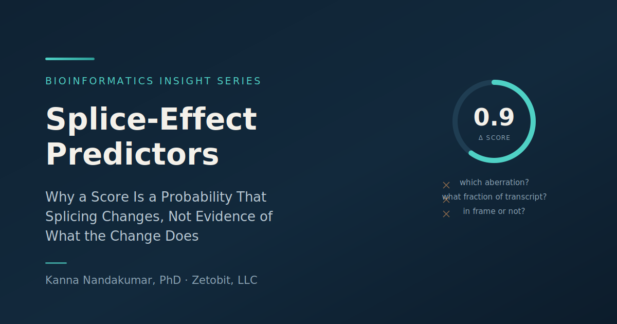
Splice-Effect Predictors: Why a 0.9 Is a Probability, Not a Consequence
A SpliceAI delta score of 0.9 is often read as near-certainty that a variant is pathogenic through a splicing mechanism. It isn't that. The score estimates the probability that splicing is altered — whether the transcript changes, not what the changed transcript is, what fraction of the mRNA pool carries it, or whether the protein breaks. The threshold at which the score becomes evidence isn't a property of the tool either: ClinGen SVI calibrated PP3 at 0.2 and BP4 at 0.1, the RUNX1 expert panel uses 0.38, an NF1 evaluation found 0.22, and deep intronic sensitivity at 0.5 was originally just 41%.
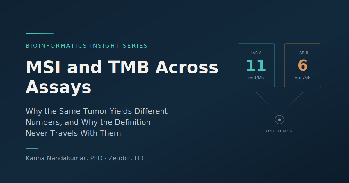
MSI and TMB Across Assays: Why the Same Tumor Yields Different Numbers
Two laboratories receive tissue from the same block. One reports a TMB of 11 mutations per megabase; the other reports 6. Neither made an error. TMB is not a physical property measured with differing precision — it's a quantity constructed from a definition that includes which territory was sequenced, which variant classes were counted, how germline was removed, and what the denominator was. Change any of those and the number changes legitimately. When 16 laboratories ran the same 29 samples, a calibration tool fixed most of the spread — which is the strongest possible evidence that nobody was wrong and nobody was measuring the same thing.
FFPE Artifacts as a Pre-Analytic Axis: Why a Low-VAF C>T Call Cannot Be Read as Biology
Formalin fixation is a chemical reaction performed on the specimen before any sequencing decision is made. It deaminates cytosine, and the resulting C>T changes arrive at the variant caller as ordinary reads with ordinary quality scores — a mutation that happened in a cassette rather than in a patient. Nothing malfunctions when they're called. The consequence reaches past a few spurious variants: because the artifact concentrates in one substitution class at low allele fraction, it lands on the measurements that sum over exactly that territory. One clinical panel needed a 10% VAF cut-off for FFPE against 5% for frozen. In one colorectal sample, unrepaired DNA gave 8.3% unstable microsatellite sites against 0.23% repaired — across a 3.5% MSI threshold.
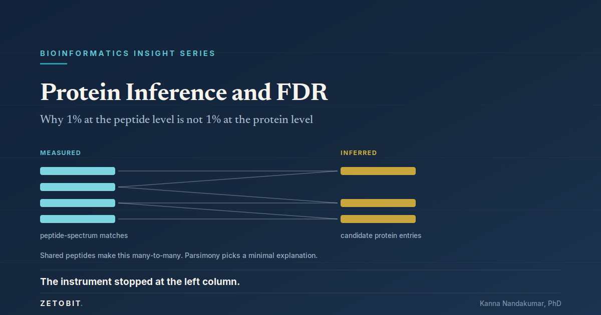
Protein Inference and FDR: Why 1% at the Peptide Level Is Not 1% at the Protein Level
A bottom-up proteomics experiment digests proteins into peptides, discards the protein-level context, measures the peptides, then reconstructs which proteins were present. That reconstruction isn't bookkeeping — peptides map to proteins many-to-many, and recovering a protein list means choosing among explanations the data doesn't fully distinguish. Parsimony resolves it with a rule, not a measurement. And the "1% FDR" in most methods sections controls the peptide layer, not the protein one: Mascot's own documentation shows a 1% sequence FDR yielding 4.55% protein FDR in the same search. The gap grows as experiments get larger.
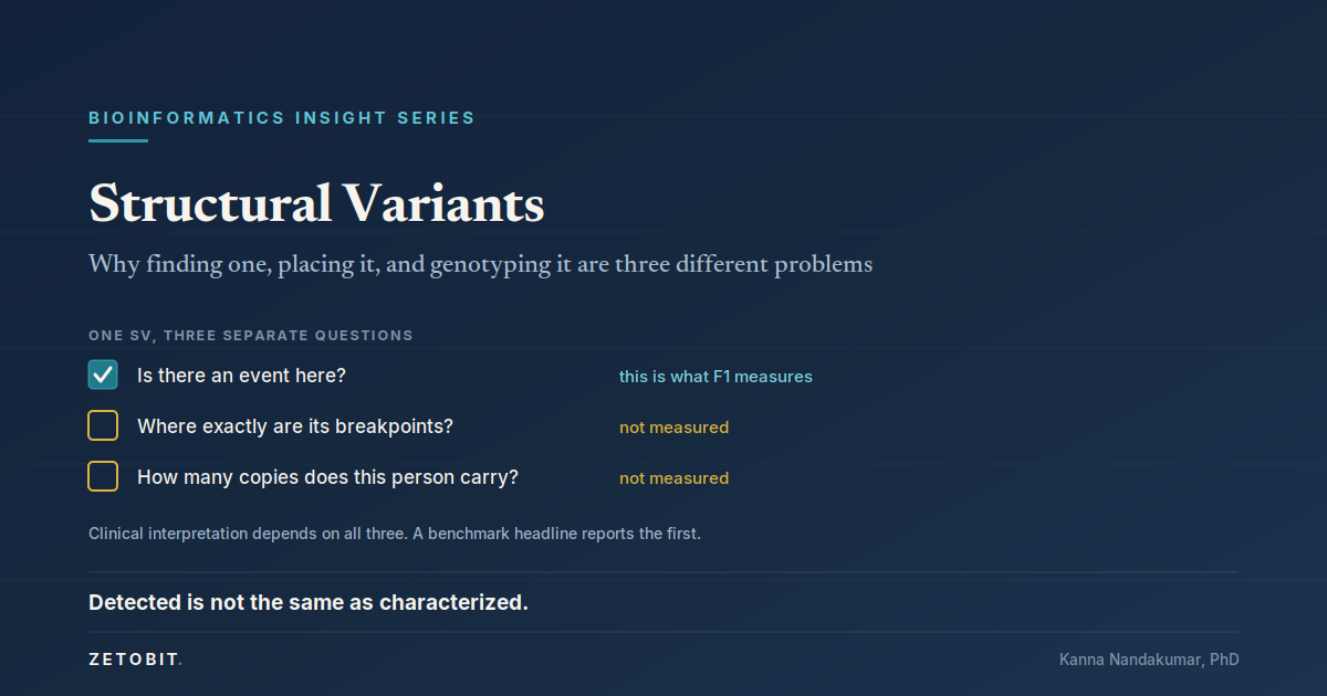
Structural Variants: Why Finding One, Placing It, and Genotyping It Are Three Different Problems
For a SNV, "detected" and "characterized" are nearly the same thing. An SV call is a composite claim: an event of some type exists, spanning roughly this interval, with breakpoints here, in this many copies. A pipeline can be right about the first part and wrong about the rest — and the standard F1 score won't distinguish those cases, because SV benchmarking counts a call correct when it lands within a tolerance window. In multi-sample data, genotypers whose detection F1 spanned 0.605 to 0.948 had genotype concordance ranging from 33.8% to 84.9%. Report all three properties, not one.
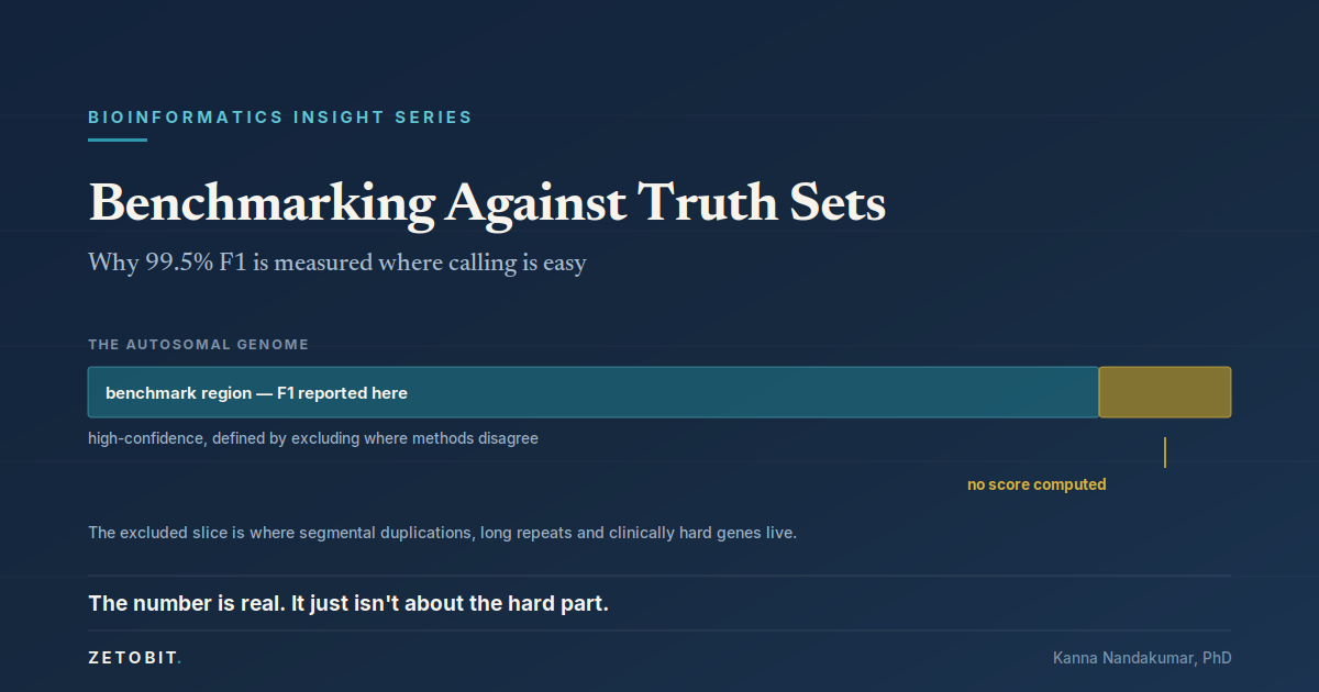
Benchmarking Against Truth Sets: Why 99.5% F1 Is Measured Where Calling Is Easy
Validating a variant caller has a standard form: run it on HG002, compare against the GIAB benchmark, report F1. The number comes back around 99.5% and the pipeline is documented as accurate. Accurate where? The comparison is restricted to high-confidence regions — regions defined partly by excluding places where methods systematically disagree, which is precisely where calling is hardest. The clearest evidence: expanding the benchmark from v3.3.2 to v4.2.1 revealed eight times more false negatives in an unchanged call set. The pipeline didn't change. The measured territory did.
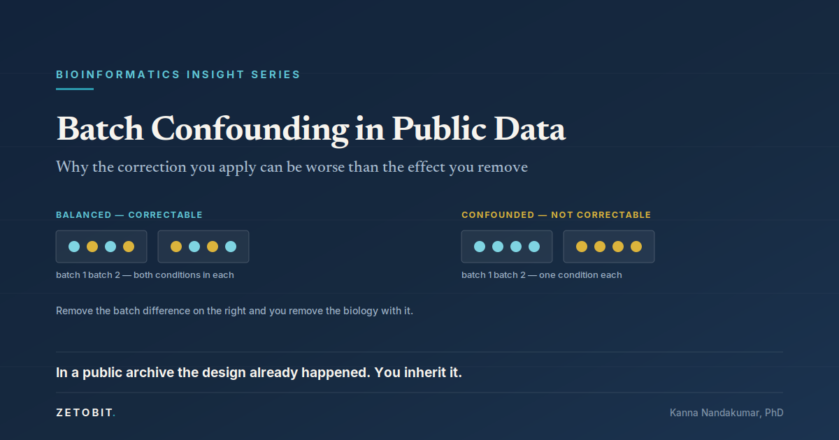
Batch Confounding in Public Data: Why the Correction You Apply Can Be Worse Than the Effect You Remove
Public archives put molecular data from tens of thousands of patients into open hands. What you can't download is the experimental design — someone else decided which samples went on which plate, which center sequenced what, and those choices are now fixed. When batch is independent of the biology, it's a nuisance you can model. When batch correlates with the variable of interest, the two occupy the same statistical space and no correction can separate them. Worse, correction applied to a confounded design can inflate significance: in one documented case, from 11 differentially expressed probesets to over 1,000 on the same data.
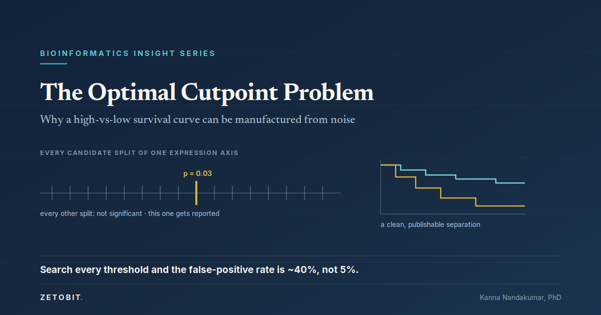
The Optimal Cutpoint Problem: Why a High-vs-Low Survival Curve Can Be Manufactured From Noise
A two-curve Kaplan-Meier plot communicates a clinical claim in a single image. It also requires a decision the data doesn't supply: gene expression is continuous, the log-rank test compares groups, so someone chose a number and called everything above it "high." If that number was chosen by searching every threshold for the smallest p-value, the false-positive rate is around 40% rather than 5%, and a reported p = 0.002 corresponds to a genuine p = 0.05. The resulting figure is visually identical to one from a pre-specified split. Nothing in it records how many splits were tried.
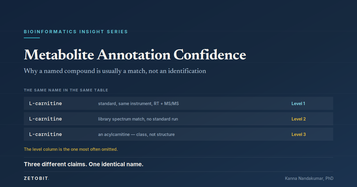
Metabolite Annotation Confidence: Why a Named Compound Is Usually a Match, Not an Identification
A metabolomics results table looks like the least ambiguous output in omics — not a p-value or a score, but a chemical name. What the instrument actually produces is a mass, a retention time, and sometimes a fragmentation spectrum. The name is assigned afterward, and the evidence behind it ranges from a compound verified against a physical standard on the same instrument to a library spectrum that merely resembled the signal. The MSI confidence levels exist to make that difference visible. The field's own assessment is that they're applied infrequently and inconsistently — and the level is the column most often missing.
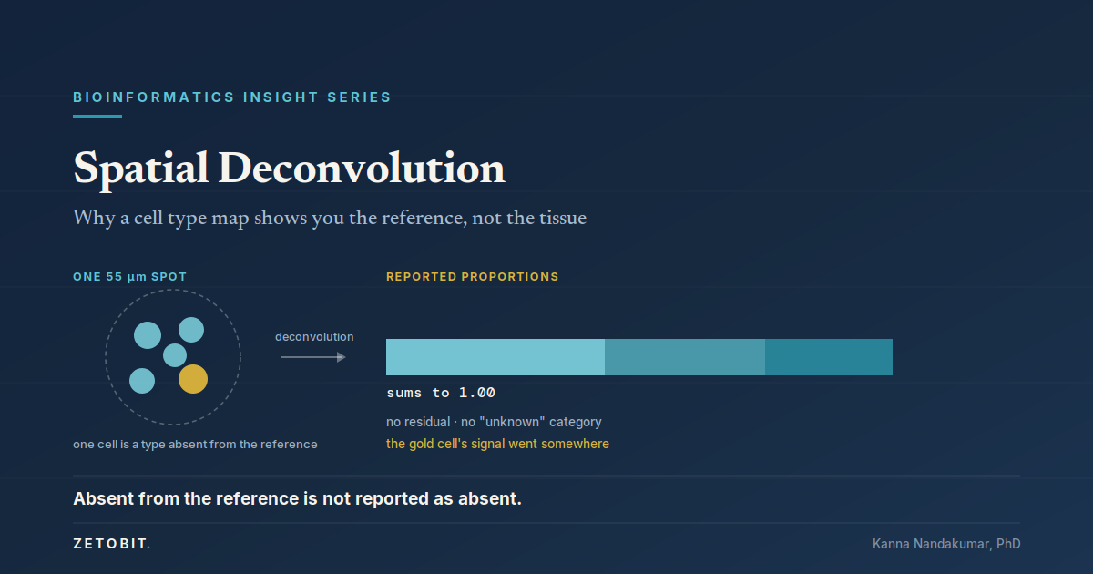
Spatial Deconvolution: Why a Cell Type Map Shows You the Reference, Not the Tissue
Spatial transcriptomics produces the most persuasive figure in modern genomics: cell types laid over real tissue architecture, looking like a photograph of where cells are. It's a model output. A Visium spot is 55 µm across and captures 1–10 cells, so every cell type map is a deconvolution against a single-cell reference — and because proportions must sum to one, a cell type absent from that reference is never reported as missing. Its signal is absorbed into whatever resembles it, inflating populations that are genuinely present. This piece covers the constraint, the dissociation bias behind it, and why the residual is where the absence becomes visible.
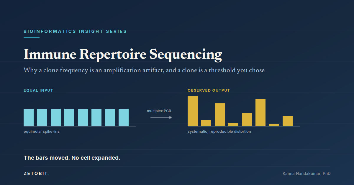
Immune Repertoire Sequencing: Why a Clone Frequency Is an Amplification Artifact and a Clone Is a Threshold You Chose
TCR and BCR sequencing produce two numbers that look like counts: how many clones are present, and how big each one is. Both are reconstructions. Using synthetic spike-ins, one study found multiplex PCR primer bias left antibody frequencies only 42–62% accurate — and the bias is systematic, so replicates agree while different primer sets correlate at R² = 0.08. Sequencing error inflated diversity estimates up to 5000-fold. And for B cells, somatic hypermutation means "the same clone" is a clustering threshold the analyst sets. This piece covers all four transformations between a cell in tissue and a percentage in a report.
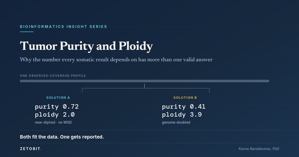
Tumor Purity and Ploidy: Why the Number Every Somatic Result Depends On Has More Than One Valid Answer
A tumor report is full of numbers that look like observations: copy number 4 at ERBB2, this mutation is clonal, TMB of 11. Almost none are read off the data. They're computed downstream of two parameters — tumor purity and ploidy — that are fit jointly from coverage in a model where different combinations explain the observations equally well. A tumor at 72% purity with a diploid genome and one at 41% purity that doubled its genome look remarkably similar. The algorithm picks one. That choice sets every copy number, every cancer cell fraction, and whether the report says whole-genome doubling occurred.
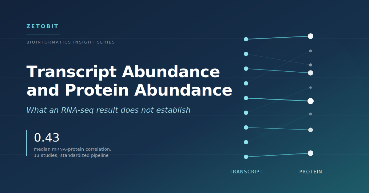
Transcript Abundance and Protein Abundance: What an RNA-Seq Result Does Not Establish
Differential expression results are routinely discussed in terms of proteins — a pathway activated, an enzyme upregulated. Across thirteen large proteogenomic studies recalculated under a single standardized pipeline, the median mRNA–protein correlation is 0.43. But the more consequential finding is why it falls short: protein measurement reproducibility alone explains 14–23% of the variance in that correlation, and adjusting for it dissolves the widely cited claim that metabolic pathways are less post-transcriptionally regulated. Some of what the field read as biology was instrument behavior. This piece separates the two, and sets out what an RNA-seq result does and does not establish about protein.
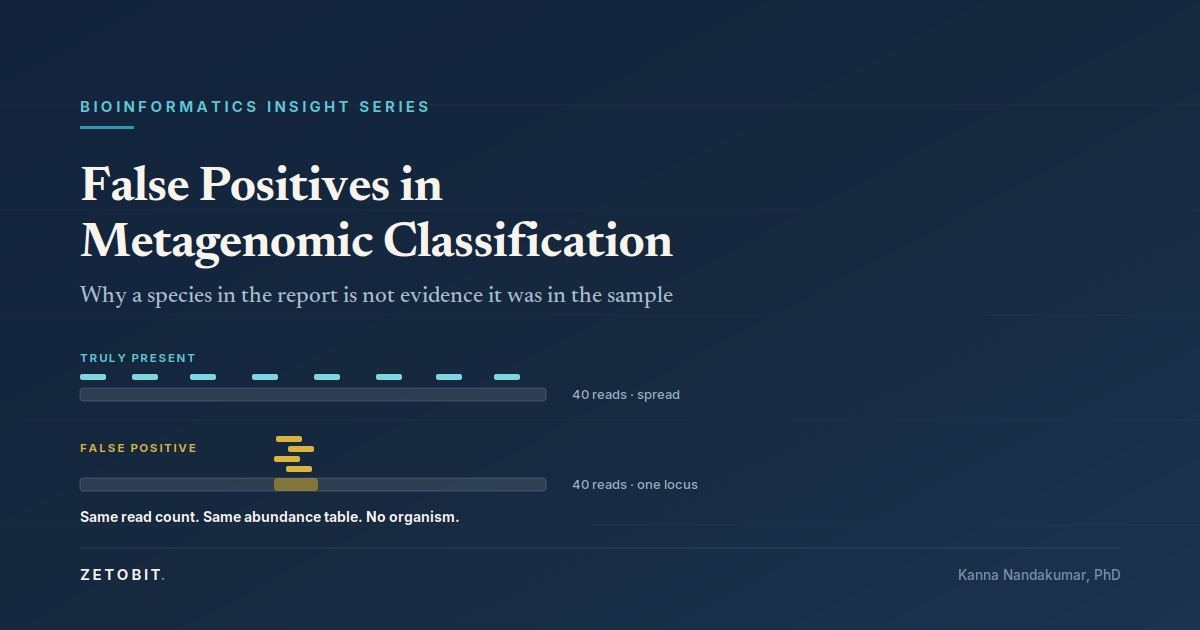
False Positives in Metagenomic Classification: Why a Species in the Report Is Not Evidence It Was in the Sample
A metagenomic classifier assigns every read the best available label from its reference database. It has no category for organisms it has never seen and no mechanism for reporting that nothing matched well. In 2020, a group swapped a fungal database for one containing frogs, snakes, and crocodiles, reran 38 human stool metagenomes, and the pipeline dutifully reported turtles and bull frogs as abundant gut taxa. Nothing malfunctioned. This piece covers the closed-world problem, why kit contamination dominates low-biomass specimens, and why coverage breadth — not read count — is what separates a detection from an artifact.
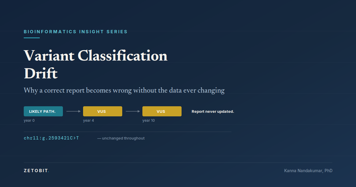
Variant Classification Drift: Why a Correct Report Becomes Wrong Without the Data Ever Changing
A pathogenicity classification is not a property of a variant. It is a statement about the evidence available on the date it was made. The sequence is permanent; the interpretation has a shelf life, and nothing in the pipeline announces when it expires. In one cohort of inherited arrhythmia variants reanalyzed a decade later, 71.87% changed classification — and the dominant movement was confident calls dissolving back into uncertainty, not the reverse. This piece covers how reclassification behaves differently by clinical indication, why laboratory-initiated reanalysis is the only mechanism that reaches cases, and what architecture makes reanalysis a query instead of a project.
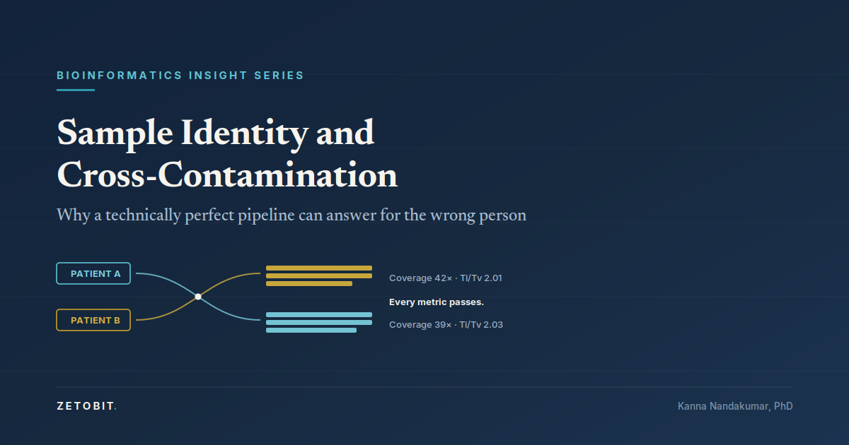
Sample Identity and Cross-Contamination: Why a Technically Perfect Pipeline Can Answer for the Wrong Person
Coverage, duplication rate, mapping rate, Ti/Tv — every standard QC metric asks whether sequencing data is good. None asks whose data it is. A swapped sample produces a beautifully clean BAM and a variant call set that passes every filter, having answered a well-posed question about the wrong person. Published estimates put the sample identity error rate between roughly 0.2% and 6%, and index hopping on patterned flow cells adds contamination the instrument creates itself. This piece covers the failure modes, why sub-1% contamination can manufacture a fusion call, and what identity QC requires that quality QC structurally cannot provide.
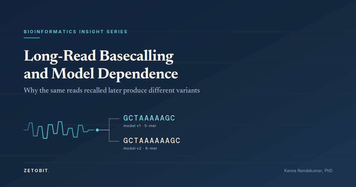
Long-Read Basecalling and Model Dependence: Why the Same Reads Recalled Later Produce Different Variants
In short-read sequencing, the FASTQ is close to a measurement. In nanopore sequencing, it is an inference — a neural network's best guess at what sequence produced an electrical trace. Reprocess a 2023 dataset with a current basecalling model and the variant list changes, even though the raw signal never did. Homopolymer lengths shift. Substitutions at methylated motifs appear and disappear, systematically, in ways depth cannot rescue. This piece examines where long-read basecalls actually come from, why model version and accuracy tier are scientific parameters rather than compute choices, and what provenance discipline long-read pipelines require that short-read pipelines do not.